[Mathematics] Linear equation: slope-intercept form

Slope-intercept form
Linear equation are any function that can be expressed in this form (named slope-intercept form)

y=mx+b

where m is the slope and b is y-intercept. if we plot the function on graph you would found it's a straight line:

This is an image from Math is fun website, since this function is a straight line so let use this graph to found out the function in slope-intercept form.
Step 1)
Let pick 2 points from the graph to found out slope the line. I select points (0,1) and (1,3):

Use the formula m

 Use slope formula found out the slope:

put x1=0,  x2=1, y2=3,  y1=1 into the formula:

we get slope of this line is 2.

Step 2) find out the y-intercept, it's 1 in this graph

Step 3) put m=2 (slope =2) and b=1 (y-intercept=1) into the formula y=mx+b, we would get

y=2+1

so the function of this line is y=2x+1.

Reference:

Image from :
https://www.mathsisfun.com/algebra/linear-equations.html
https://www.pinterest.com/pin/651473902321977776/

[Mathematics] Type and notation of interval

In mathematics, a (real) interval is a set of real numbers lying between two numbers, we used to see something like this:

x < 4

it means x is smaller than 4.

-2 ≤ x ≤ 3

and this mean x is greater or equal to -2 and less than or equal to 3.

Types of the interval :

• close-interval
• open-interval, doesn't not 
• half-interval
• infinite interval 

Close interval

we use the notation [ or ] to represent the closed side

[-2,3] means -2 ≤ x ≤ 3

Open interval

we use the notation ( or ) to represent the open side

(-16,-9) means -16 < x < -9

Half interval

you would have both open side and close side in the interval.

[-7,2) means -7 ≤ x < 2

Infinite interval

For infinite interval, the ∞ sign is used.

(1,∞ ) mean x>1

More usage and example:

http://www.csgnetwork.com/directintervalcalc.html

Remarks

Sometimes we use the union notation ⋃ to join two interval"

(-∞,1)⋃[∞,2)

(-∞,1) means interval x<1 and [∞,2) means interval x≥ 2.

(-∞,1)⋃(∞,2) is equivalent to x<1 or x≥ 2.

and intersect notation ∩ to get the collection of values in both interval:

(-∞,2)∩[1,3)

(-∞,2) means interval x<2 and [1,3) means interval 1≤x<3.

(-∞,2)∩[1,3) is equivalent to 1≤x<2.

Reference:

https://en.wikipedia.org/wiki/Interval_(mathematics)

https://wikidiff.com/interval/range

[Mathematics] Linear equation: two-point equation

Although slope-intercept form is more common to find out the function of a linear equation, we can also use another method named "2 points equation" to get the function.
The advantage using this method is you don not need to know the slope.

Read more about slope-intercept form :
[Mathematics] Linear equation: slope-intercept form

equation of two-point equation:

where (x₁ , y₁) and (x₂ , y₂) are points on the line.

Let use this graph as example, we pick out 2 points (0,1) and (1,3) on the line:

put x₁ = 0, y₁ =1, x₂ =1, y₂=3 into the equation:

And here we got the function y=2x+1

[Mathematics] Symmetric with respect to axis

There are 3 major type of symmetric about an axis:

1. symmetric with respect to the x-axis
2. symmetric with respect to the y-axis
3. symmetric with respect to the the origin

The advantage to know an equation is symmetric is you can use the result to predict behavior on the other side.

In addition to using graph to find out the function is symmetric with respect to axis, we can also use check it symmetric alone axis by replacing points.

Let use this function as example:

y²=x-1

Examine symmetric about y-axis
We can replace (x,y) with (-x,y) to examine symmetric about y-axis
By replacing x to -x, we get y²=(-x)-1 from y=x-1

y²=-x-1

Since y²=-x-1 is not same to y²=x-1, the graph would not symmetric about y-axis.


Examine symmetric about x-axis
We can replace (x,y) with (x,-y) to examine symmetric about x-axis
By replacing y to -y, we get -y²=x-1 from y²=x-1

(-y)²=x-1
 (y)²=x-1

Since (-y)²=x-1 is same to y²=x-1, the graph is symmetric about x-axis.


Examine symmetric about origin
We can replace (x,y) with (-x,-y) to examine symmetric about origin
By replacing y to -y, we get (-y)²=(-x)-1 from y²=x-1

(-y)²=(-x)-1
    y²=-x-1

Since (-y)²=(-x)-1 is not same to y²=x-1, the graph is not symmetric about origin.

Finally, let take a peek about how y2=x-1 look like in graph:

[graph][example] graph vertix, edge, degree etc

Defination

point  : A particular position which is usually represted by a dot: whether in a one-dimensional, two-dimensional, or three-dimensional space.
line   : The notion of line or straight line between 2 points.
vertex : A vertex is a point where multiple lines meet, it's also so-called node.
edge   : An edge is a particular type of line segment joining two vertices, sometimes we call it path.
adjacent edge   : two different edges have both vertices common.
adjacent vertex : two different verteix have both edges common.
loop   : loop is an edge is drawn from vertex to itself.
degree of a vertex : The degree of a vertex is the number of edges incident with that vertex.
Degree Sequence: Degree sequence of a graph is the list of degree of all the vertices of the graph
indegree  : Indegree of vertex V is the number of edges which are coming into the vertex V.
outdegree : Outdegree is the number of edges which are going out from the vertex V.
isolated vertex  : A vertex without any indegree and outdregree.
parallel edges   : A pair of vertices is connected by more than one edge, these edges are parallel edges.
directed edge    : means the edges have an orientation which is represented by an arrow: the tail and head of this arrow are the nodes representing the beginning and ending points of the edge.
undirected graph : An undirected graph has no directed edges.
directed graph   : An directed graph has directed edges.
Pendant point    : vertex (also leaf vertex) is a vertex with only degree one.

Undirected graph

vertices : {a,b,c,d}
edges    : {ab,ab,bc,cd,bd}
adjacent edges 
 - adjacent edge of vertix "a" are {ab1,ab2}
 - adjacent edge of vertix "b" are {ab1,ab2,cb,bd}
 - adjacent edge of vertix "c" are {cb,cd}
 - adjacent edge of vertix "d" are {bd,bc}
adjacent vertex:
 - adjacent vertex of edge ab1 and ab2 is a.
 - adjacent vertex of edge {ab1,ab2,cd,bd} is b.
 - adjacent vertex of edge bc and bd is c.
 - adjacent vertex of edge cd and bd is d.

(Remark. The figure above is a multi graph.)

 

Vertex    Connecting to      Degree
-------------------------------------
  a          b              deg(a) = 2
  b          a,c,d         deg(b) = 2
  c          c,b           deg(c) = 4
  d          b,c           deg(d) = 2

 

from this table we can found the degree sequence of {a,b,c,d} is {2,4,2,2}

 

 

---

Directed graph

vertices                 : {A,B,C,D,E,F,G,H<I,J}
edges                     : {AD,DF,DG,DH,BD,BE,EG,CE,CH}
pandent vertices  : {A,F,J}
isolated vertex     : {I,J}
loop                       : {J}

 

Vertex   in-degree  out-degree
------------------------------
  A          0           1
  B          0           2
  C          0           2
  D          2           3
  E          2            1
  F          1            0
  G         2            0
  H         2            0
  I          0            0
  J          1            1

 

adjacent edges :
 - adjacent edge of vertix B are {BD,BE}
 - adjacent edge of vertix C are {CE,CH}
 - adjacent edge of vertix D are {AD,BD,DF,DG,DH}
 - adjacent edge of vertix E are {BE,EG}
 - adjacent edge of vertix G are {DG,EG}
 - adjacent edge of vertix H are {DH,CH}

 

adjacent vertex:
 - adjacent vertex of edge {AD,BD,DH,DG,DF) is vertix D.
 - adjacent vertex of edge {BE,EG,CE} is E.
 - adjacent vertex of edge {CH,DH} is H.
 - adjacent vertex of edge {DG,EG} is G.

 

---

Reference:

http://mathworld.wolfram.com/PendantVertex.html
https://en.wikipedia.org/wiki/Vertex_(graph_theory)
https://www.tutorialspoint.com/graph_theory/graph_theory_fundamentals.htm
https://www.math.cuhk.edu.hk/~wei/ch2.pdf
https://en.wikipedia.org/wiki/Loop_(graph_theory)
https://www.quora.com/When-are-two-edges-said-to-be-adjacent-in-graph-theory
http://rosalind.info/glossary/directed-edge/
http://www.people.vcu.edu/~gasmerom/MAT131/graphs.html

[JavaScript][Example] get median from a list of numbers

<script>
const ROUND_TO_FIXED = 2;
function _stringToList(string){
    return string.split(",");
}
function _roundToFixed(num){
    return Number(parseFloat(num).toFixed(ROUND_TO_FIXED));
}
function getSampleMedian(string){
    var sourceList  = _stringToList(string);
    var sortedList  = sourceList.sort();
    var medianPos   = null;
    var medianIndex = null;
    var median      = 0;
    if(sortedList.length%2 === 0){
        medianPos   = (sortedList.length+1)/2;
        medianIndex = medianPos-1;
        median      = ( parseFloat(sortedList[Math.ceil(medianIndex)]) +
                        parseFloat(sortedList[Math.floor(medianIndex)]) ) /2;
    }else{
        medianPos   = (sortedList.length+1)/2;
        medianIndex = medianPos -1;
        median      = sortedList[medianIndex];
    }
    return median;
}
var testValue = "1,2,3,5,1,2,6";
console.log(getSampleMedian(testValue));
</script>

Result :
2

[JavaScript][Example] get mode from a list of numbers

This post mark down the logic using javaSrcipt get the modes, source samples are with string data type and separated by comma.

<script>
const ROUND_TO_FIXED = 2;
function _stringToList(string){
    return string.split(",");
}
function _roundToFixed(num){
    return Number(parseFloat(num).toFixed(ROUND_TO_FIXED));
}
function getSampleModes(string){
    var sourceList  = _stringToList(string);
    var max         = -Infinity, x;
    var json        = {},
        frequencies = {}
    var modes       = [];
    //Records the occurs of numbers
    for(var key in sourceList){
        if(! (sourceList[key] in frequencies)){
            frequencies[sourceList[key]] = 1;
        }else{
            frequencies[sourceList[key]] += 1;
        }
    }
    // Get modes
    for(var key in frequencies) {
       if( frequencies[key] > max) max = frequencies[key];
       if( frequencies[key] == max) modes.push(key);
    }
    return modes;
}
var source = "1,2,3,5,1,2,6"
console.log(getSampleModes(source));
</script>

Result

Refercene:
https://en.wikipedia.org/wiki/Mode_(statistics)

 

[JavaScript][Example] get simple mean from a list of numbers

This post mark down the logic using javaSrcipt execute simply mean calaulation.
source samples are with string data type and separated by comma.
using this formula :

<script>
const ROUND_TO_FIXED = 2;
function _stringToList(string){
    return string.split(",");
}
function _roundToFixed(num){
    return Number(parseFloat(num).toFixed(ROUND_TO_FIXED));
}
function getSampleMean(string){
    var sourceList = _stringToList(string),
        sum        = 0;
    for(var i in sourceList){
        sum += parseFloat(sourceList[i]);
    }
    return _roundToFixed(sum / sourceList.length);
}
var source = "1,2,3,5,1,2,6"
console.log(getSampleMean(source));
</script>

Result:
2.86

Reference:
https://en.wikipedia.org/wiki/Mean
https://www.w3schools.com/Js/js_json_parse.asp
https://stackoverflow.com/questions/9907419/how-to-get-a-key-in-a-javascript-object-by-its-value

[tutorial][python] Determinant matrix

It’s for help us to found out inverse of a matrix. syntax like this


And matrix to use determinant MUST BE square (i.e. have the same number of rows as columns).

You better if have a look of this link:
https://www.mathsisfun.com/algebra/matrix-determinant.html

Example 1

Using determinant to calculate this matrix :

We use this rule to multiply elements in matrix where Blue is positive (+ad) and Red is negative (−bc) :


With python, we can use det() method to get the result.

import numpy as np
from scipy import linalg as la

A = np.array([[3,8],[4,6]])
print(la.det(A))

Result :

-14.0

Example 2

det(A) = | A | = (1*4)-(2*3) = 4 - 6  = - 2.0

Calculation with python :

import numpy as np
from scipy import linalg as la

A = np.array([[1,2],[3,4]])
print(A)
B = la.det(A)
print(B)

Result :

[[1 2]
 [3 4]]
-2.0

Example 3

Let use python with package numpy and linalg to represent the determinant of this 3×3 matrix:

import numpy as np
from scipy import linalg as la

A = np.array([[6,1,1],[4,-2,5],[2,8,7]])
print(A)
B = la.det(A)
print(B)

Result: 

[[ 6  1  1]
 [ 4 -2  5]
 [ 2  8  7]]
-306.0

[tutorial][python] Matrix of ones

All elements in matrix are number 1, that’s so called Matrix of ones.

Reference:
https://en.wikipedia.org/wiki/Matrix_of_ones

Calculation with python:

A = np.array([[13,9,7],[8,7,4],[6,4,0]])
B = np.array([[1,1,1],[1,1,1],[1,1,1]])
print(A.dot(B))

Result :

[[29 29 29]
 [19 19 19]
 [10 10 10]]

It’s special that elements in 1st line in output matrix are all values 13+9+7 = 29, it’s the amount of the 1st line in  input elements.

All elements in 2nd lines of output matrix valued 19, which’s the amount of the 2nd line in  input elements (8+7+4).

All elements in 3rd lines of output matrix valued 10, which’s the amount of the 2rd line in  input elements (6+4+0).

[tutorial][python] Zero Matrix

By using zero matrix, all result would turn to 0

Calculation with python:

import numpy as np
from scipy import linalg

A = np.array([[13,9,7],[8,7,4],[6,4,0]])
B = np.array([[0,0,0],[0,0,0],[0,0,0]])
print(A.dot(B))

Result:

[[0 0 0]
 [0 0 0]
 [0 0 0]]

Using numpy to create zero matrix:

import numpy as np

a = np.zeros((10,3))
print(a)
print("--------------")
b = a.T
print(b)
print("--------------")
c = np.reshape(b,(5,6))
print(c)

Result :

[[ 0.  0.  0.]
 [ 0.  0.  0.]
 [ 0.  0.  0.]
 [ 0.  0.  0.]
 [ 0.  0.  0.]
 [ 0.  0.  0.]
 [ 0.  0.  0.]
 [ 0.  0.  0.]
 [ 0.  0.  0.]
 [ 0.  0.  0.]]
--------------
[[ 0.  0.  0.  0.  0.  0.  0.  0.  0.  0.]
 [ 0.  0.  0.  0.  0.  0.  0.  0.  0.  0.]
 [ 0.  0.  0.  0.  0.  0.  0.  0.  0.  0.]]
--------------
[[ 0.  0.  0.  0.  0.  0.]
 [ 0.  0.  0.  0.  0.  0.]
 [ 0.  0.  0.  0.  0.  0.]
 [ 0.  0.  0.  0.  0.  0.]
 [ 0.  0.  0.  0.  0.  0.]]

[tutoral][python] Identity Matrix

The identity matrix [I] for multiplication is a square matrix with a 1 for every element of the principal diagonal (top left to bottom right) and 0 in other position:

It is a special matrix, because when we multiply by it, the original is unchanged:

Let prove A*I = A in Python:

import numpy as np
from scipy import linalg

A = np.array([[13,9,7],[8,7,4],[6,4,0]])
B = np.array([[1,0,0],[0,1,0],[0,0,1]])
print(A.dot(B))

Result:

[[13  9  7]
 [ 8  7  4]
 [ 6  4  0]]

And then I*A = A ?

import numpy as np
from scipy import linalg

A = np.array([[1,0,0],[0,1,0],[0,0,1]])
B = np.array([[13,9,7],[8,7,4],[6,4,0]])
print(A.dot(B))

Result:

[[13  9  7]
 [ 8  7  4]
 [ 6  4  0]]

Orz, the result really same.

Reference :
https://www.mathsisfun.com/algebra/matrix-multiplying.html

[Tutorial][Python] Multiplying a Matrix by Another Matrix

Suppose there are 2 matrix for multiplication: This is the most basic method to do matrix calculation. In example shown below, 2 is so called scalar in this calculation. We multiply each number in matrix by this scalar 2, and mark multiplied result in same location in matrix.

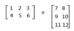
*The number of columns in A need to equal to the number of rows in B.
To calculate that we need to do an action named “dot product”
 

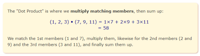
 With python, we can use .dot() to calculate the dot product for these 2 matrix:



Example for Multiplying a Matrix by Another Matrix

Question 1) 

4*1+5*0 = 4+0 = 4
Result is 4

Python :

import numpy as np
from scipy import linalg

A = np.array([4,5])
B = np.array([[1],[0]])
print(A.dot(B))

Result:

[4]

Question 2

From a to f in order, there are the calculation order with use dot product :

a: (1,-2) • (4,-1)  = (1*4)+(-2*-1)  = 4+2 = 6
b: (0,3) • (4,-1)  = (0*4)+(3*-1)   = 0-3 = -3
c: (-1,4) • (4,-1) = (-1*4)+(4*-1)  = -4-4 = -8
d: (1,3) • (1,2)   = (1*4)+(-2*-1)  = 1-4 = -3
e: (0,3) • (1,2)   = (0*4)+(3*-1)   = 0+6 = 6
f: (-1,4) • (1,2)  = (-1*4)+(4*-1)  = -1+8 = 7

Calculation with Python:

import numpy as np
from scipy import linalg

A = np.array([[1,-2],[0,3],[-1,4]])
B = np.array([[4,1],[-1,2]])
print(A.dot(B))

Result :

[4]

Reference:
http://chortle.ccsu.edu/vectorlessons/vmch15/vmch15_4.html


Question 3
This is a question from Math is fun website:
https://www.mathsisfun.com/algebra/matrix-multiplying.html

From information, i create 2 matrix:

And the result would be in this format: [a,b,c,d]

a.        (3,4,2) • (13,8,6)   = (3*13)+(4*8)+(2*6)  = 39+32+12 = 83
b.        (3,4,2) • (9,7,4)     = (3*9)+(4*7)+(2*4)    = 27+28+8   = 63
c.        (3,4,2) • (7,4,0)     = (3*7)+(4*4)+(2*0)    = 21+16+0   = 22
d.        (3,4,2) • (15,6,3)   = (3*15)+(4*6)+(2*3)  = 45+24+6   = 75

Result is [$83,$63,$22,$75], which’s means
A.        Sold are monday are $83.
B.        Sold are Tuesday are $63.
C.        Sold are Wedenday are $22.
D.        Sold are Thurday are $75.

Calculation with Python:

import numpy as np
from scipy import linalg

A = np.array([3,4,2])
B = np.array([[13,9,7,15],[8,7,4,6],[6,4,0,3]])
print(A.dot(B))

Result

[83 63 37 75]

Reference:
http://chortle.ccsu.edu/vectorlessons/vmch15/vmch15_4.html
https://www.mathsisfun.com/algebra/matrix-multiplying.html

[Tutorial][python] Scalar multiplication

This is the most basic method to do matrix calculation. In example shown below, 2 is so called scalar in this calculation. We multiply each number in matrix by this scalar 2, and mark multiplied result in same location in matrix.

With python, we can use .dot() to calculate the dot product for this matrix with scalar 2:

import numpy as np
from scipy import linalg
A = np.array([[4,0],[1,-9]])
print(A.dot(2))

Result :

[[ 8 0]
[ 2 -18]]

[tutorial][python] Using numpy module create matrix

1) import numpy as np is for creating numpy object.
2) np.arange(25) is for creating a list from 0 to 24, total is 25 elements.
3) a.reshape((5,5)) means from the list (data source) provided, create a 5*5 array.

Python example:

import numpy as np #1
a = np.arange(25) #2
b = np.arange(25)
print("------- Source -------")
print(a)
print(b)
print("------- Reshape ------")
a = a.reshape((5,5)) #3
b = b.reshape((5,5))
print(a)
print(b)
print("--- After calculation ---")
print(a+b)
print(a-b)
print(a*b)
print(a/b)
print(a**2)
print(a<b)
print(a>b)
print(a.dot(b))

Result:

------- Source -------
[ 0  1  2  3  4  5  6  7  8  9 10 11 12 13 14 15 16 17 18 19 20 21 22 23 24]
[ 0  1  2  3  4  5  6  7  8  9 10 11 12 13 14 15 16 17 18 19 20 21 22 23 24]
------- Reshape ------
[[ 0  1  2  3  4]
 [ 5  6  7  8  9]
 [10 11 12 13 14]
 [15 16 17 18 19]
 [20 21 22 23 24]]
[[ 0  1  2  3  4]
 [ 5  6  7  8  9]
 [10 11 12 13 14]
 [15 16 17 18 19]
 [20 21 22 23 24]]
--- After calculation ---
[[ 0  2  4  6  8]
 [10 12 14 16 18]
 [20 22 24 26 28]
 [30 32 34 36 38]
 [40 42 44 46 48]]
[[0 0 0 0 0]
 [0 0 0 0 0]
 [0 0 0 0 0]
 [0 0 0 0 0]
 [0 0 0 0 0]]
[[  0   1   4   9  16]
 [ 25  36  49  64  81]
 [100 121 144 169 196]
 [225 256 289 324 361]
 [400 441 484 529 576]]
[[ nan   1.   1.   1.   1.]
 [  1.   1.   1.   1.   1.]
 [  1.   1.   1.   1.   1.]
 [  1.   1.   1.   1.   1.]
 [  1.   1.   1.   1.   1.]]
[[  0   1   4   9  16]
 [ 25  36  49  64  81]
 [100 121 144 169 196]
 [225 256 289 324 361]
 [400 441 484 529 576]]
[[False False False False False]
 [False False False False False]
 [False False False False False]
 [False False False False False]
 [False False False False False]]
[[False False False False False]
 [False False False False False]
 [False False False False False]
 [False False False False False]
 [False False False False False]]
[[ 150  160  170  180  190]
 [ 400  435  470  505  540]
 [ 650  710  770  830  890]
 [ 900  985 1070 1155 1240]
 [1150 1260 1370 1480 1590]]

[python][tutorial] Eigenvalues and Eigenvectors

Example 1

 

Let use python calculate what’s the determinant of first:  

import numpy as np
from scipy import linalg as la
A = np.array([[1,2],[3,2]])
print(A)
B = la.det(A)
print(B)

Result:

[[1 2]
 [3 2]]
-4.0

 That’s means:

In this case, 4 is the eigenvalues λ

import numpy as np
from scipy import linalg as la

A = np.array([[1,5,2],[2,4,1],[3,6,2]])
lna,v = la.eig(A)
l1,l2,l3 =lna
#Eigenvalue
print(l1,l2,l3)
print("----------------")
#Eigenvector
print(v)
print("----------------")
print(v[:,0])
print(v[:,1])
print(v[:,2])
v1 = np.array(v[:,0]).T
print("----------------")
print(v1)
print(la.norm(A.dot(v1)-l1*v1))

Result:

(7.95791620491+0j) (-1.25766470568+0j) (0.299748500767+0j)
----------------
[[-0.5297175  -0.90730751  0.28380519]
 [-0.44941741  0.28662547 -0.39012063]
 [-0.71932146  0.30763439  0.87593408]]
----------------
[-0.5297175  -0.44941741 -0.71932146]
[-0.90730751  0.28662547  0.30763439]
[ 0.28380519 -0.39012063  0.87593408]
----------------
[-0.5297175  -0.44941741 -0.71932146]
3.233018248352212e-15

V[:,0] means 1st line of matrix

[tutorial][python] Inverse matrix

Inverse matrix is available in n×n matrix only. But n×n matrix may not means have inverse matrix.

If matrix A and matrix B are inverse matrix each others, it can be represented as

Suppose there are 2 matrix:
 
Let have a look how to get the result, work for a dot product on AB first:
A.      (2,3) • (-7,5) = (2*-7)+(3*5)  = -14+15 = 1
B.      (2,3) • (3,-2) = (2*3)+(3*-2) = 6-6       = 0
C.      (5,7) • (-7,5) = (5*7)+(7*5)  = -35+35 = 0
D.      (5,7) • (3,-2) = (5*3)+(7*-2) = 15-14   = 1

BA use same method to get.

Both of the them are resulted 1 , B is in inverse matrix of A and A is in inverse matrix of B. We can represent their relation in this math format :

 * Pay attention to the -1 sign.

Example 1 

The coming example use as source stored in A, and than use linalg.inv() inverse matrix of source and print it out:

import numpy as np
from scipy import linalg

A = np.array([[2,3],[5,7]])
print(A)
print(linalg.inv(A))

Result :

[[2 3]
 [5 7]]
[[-7.  3.]
 [ 5. -2.]]

Example 2

This example is to calculate dot product

(2,3) • (5,7) = 2*5 + 3*7 = 10+21 =31

import numpy as np
from scipy import linalg

A = np.array([2,3])
B = np.array([5,7])

print(A.dot(B))

Result :

31

Example 3

Example in python :

import numpy as np
from scipy import linalg

A = np.array([[1,3,4],[2,5,1],[2,3,8]])
print(A)
print(linalg.inv(A))
print(A.dot(linalg.inv(A)))

Result:

[[1 3 4]
 [2 5 1]
 [2 3 8]]
[[ -1.76190476e+00   5.71428571e-01   8.09523810e-01]
 [  6.66666667e-01   5.55111512e-17  -3.33333333e-01]
 [  1.90476190e-01  -1.42857143e-01   4.76190476e-02]]
[[  1.00000000e+00   2.22044605e-16   0.00000000e+00]
 [ -2.22044605e-16   1.00000000e+00  -2.77555756e-16]
 [  0.00000000e+00   2.22044605e-16   1.00000000e+00]]

[Tutorial] Empirical rule (68–95–99.7 rule)

If your data is with normal or nearly normal distribution, unimodal distribution which is symmetric. Empirical rule should be applied on your data.

photo from statisticshowto.com


We call location of distribution which is located at this line as μ+σ.

 

and scope in red rectangle is from μ to μ+σ

On the other hand, we call location of distribution which's located at this line as μ-σ.

and scope in red rectangle is from μ to μ-σ.

we call the location of distribution here as μ+2σ.

------------------------------------------------------------------------------
Suppose :

• X is an observation from a normally distributed random variable
• μ is the mean of the distribution
• σ is its standard deviation:

Empirical rule means

1) Around 68% of values fall within one standard deviation of the mean.

In math we use this to represent the probability a random distributed value X located between μ-σ to μ+σ :

In figure,the scope [μ-σ, μ+σ] is shown at area in blue.

2) Around 95% of the values fall within two standard deviations from the mean.

In math we use this to represent the probability a random distributed value X located between μ-2σ to μ+2σ :

 

In figure,the scope [μ-σ, μ+σ] is shown at area in blue and brown.

3) Almost all of the values — about 99.7% — fall within three standard deviations from the mean.

In math we use this to represent the probability a random distributed value X located between μ-3σ to μ+3σ :

In figure,the scope [μ-σ, μ+σ] is shown at area in blue ,brown and green.

Example

http://www.oswego.edu/~srp/stats/wts_males.htm 

Reference

http://www.statisticshowto.com/68-95-99-7-rule/
http://www.oswego.edu/~srp/stats/6895997.htm